Research talk · October 2026
Recurrent Looped
Transformer
A causal encoder and a decoder with feedback across tokens.
Press → or Space to begin · ? for help
Overview
Feed the final state into the next token
A Transformer applies a fixed number of layers to each token. RLT feeds the decoder’s final state into the next token, so the computation path grows with the sequence at a fixed per-token cost.
Unless TC⁰ = NC¹, fixed-depth Transformers cannot track S₅ compositions over arbitrarily long inputs: Merrill, Petty & Sabharwal (2024) ↗. Manuscript updated October 5, 2026.
00 · Background
Background & related work
Shared blocks across depth; persistent state across tokens.
- 01Universal Transformer: refine representations over depth.
- 02Looped Transformer: revisit a shared stack.
- 03DeepLoop: scale residuals for repeated parameter use.
- 04RLT: carry the decoder’s computation across tokens.
00 · Background
Universal Transformer: recurrent depth
Dehghani et al., Universal Transformers (2018 / ICLR 2019) ↗ · Schematic omits residual and normalization paths. Autoregressive generation still proceeds token by token.
00 · Background
Looped Transformer: reuse a stack
Parameters are stored once; computation grows with the loop count. More loops add latent refinement steps before readout.
Saunshi et al. (ICLR 2025) ↗ · Geiping et al., recurrent-depth language models (2025) ↗ · Schematic; concrete loop schedules vary.
00 · Background
DeepLoop: gradients from repeated block use
The analysis tracks repeated use of the same parameters, through a visit-alignment coefficient \(\kappa_R\).
Li, Zhang, Guo, Gu & Wang, DeepLoop (2026) ↗ · A scaling rule for weight-tied depth.
00 · Background
DeepLoop: residual and initialization scaling
\(N=KR,\qquad \alpha=(2N)^{1/2},\quad \beta=(8N)^{-1/2}\)
Li, Zhang, Guo, Gu & Wang, DeepLoop (2026) ↗ · j selects the shared physical block for unrolled visit i.
00 · Background
DeepLoop: validation loss by loop count
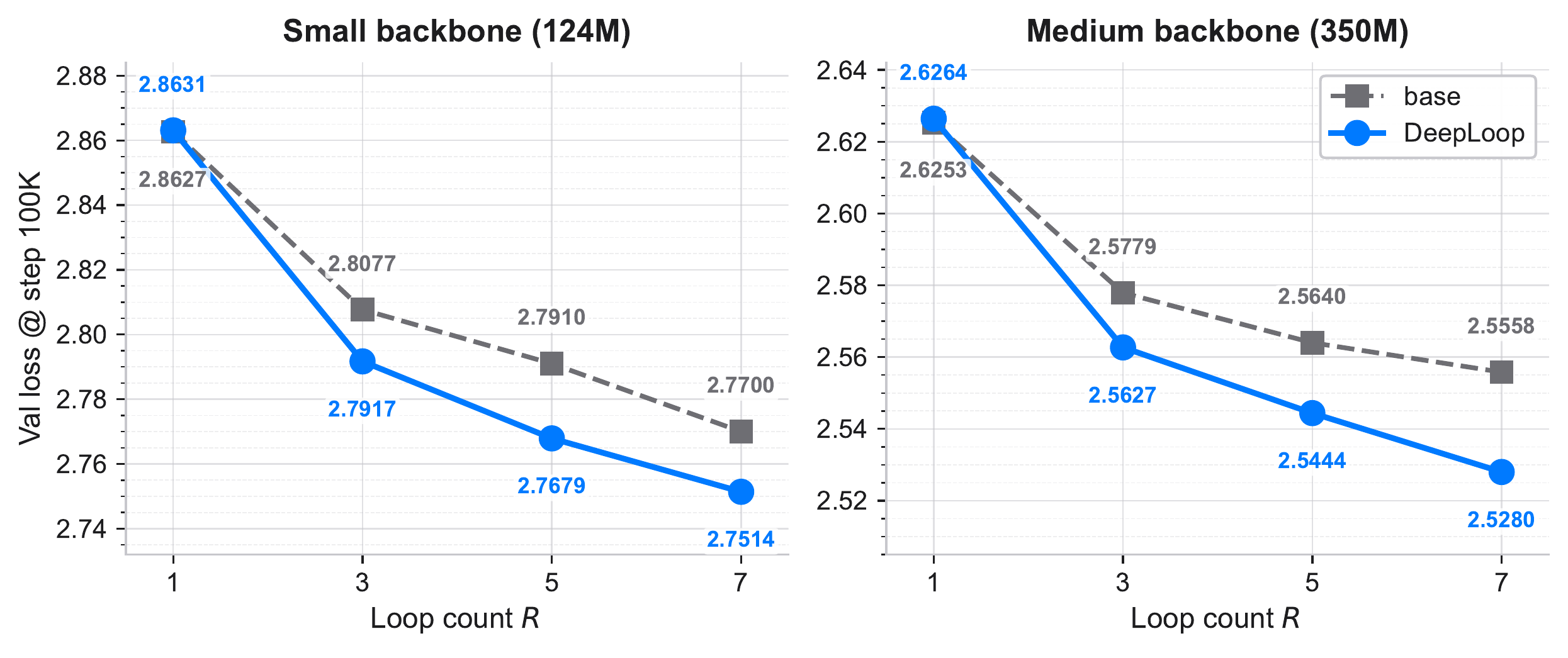
On FineWeb-Edu, DeepLoop lowers validation loss at R = 3, 5, 7 for both backbone sizes; R = 1 is essentially unchanged.
Li, Zhang, Guo, Gu & Wang, DeepLoop (2026) ↗ · Original project figure. Base: α = β = 1. Lower is better.
00 · Background
Recurrence and memory in related models
| Line of work | Reused / carried object | Connection to RLT |
|---|---|---|
| Universal / looped Transformer | Shared blocks across depth | Iterative latent computation |
| DeepLoop | Loop-aware residual scaling | Training tied depth |
| Feedback Transformer | Past representations across layers | Temporal feedback |
| Block-Recurrent / RMT | State across blocks / segments | Chunk-level memory |
| YOCO | Shared global KV memory | Reusable encoder memory |
| Coconut | Hidden state at latent positions | Continuous latent feedback |
Feedback Transformer ↗ · Block-Recurrent ↗ · RMT ↗ · YOCO ↗ · Coconut ↗
00 · Background
Depth recurrence and token recurrence
The loop index advances through repeated applications of a shared stack.
The final decoder output enters the next token update; global and local memories remain accessible.
The RLT experiments in this talk use untied encoder and decoder weights.
01 · Architecture
Encoder memory and decoder feedback
The decoder reads encoder KV memory and receives the previous token’s final hidden state.
The prompt–response boundary does not reset the hidden state or decoder caches.
Architecture
RLT-1: the complete token update
Encoder features and global memory
The final encoder output feeds both the gated merge and the global K/V projection. G = 1 shares that projected memory across decoder layers.
Per-layer local memory
Each SWA layer projects its own current KV and combines it with its own retained history.
Full-decoder feedback
The final output sₜ returns to the next token’s merge. Orange marks the one-token delay.
Manuscript architecture diagram. Arrows run upward within each stack; every + is a residual addition.
RLT-1
The state includes the attention caches
After an update, each decoder layer retains at most W − 1 past positions.
Architecture
Encoder features and shared KV memory
Causal encoder stack
After embedding, each encoder layer applies causal self-attention and an FFN, with a residual addition after each sublayer.
Two uses of the same eₜ
One path enters the recurrent merge. The other normalizes and projects eₜ into global keys and values.
Prefix-restricted reads
Append (kₜ, vₜ) to M≤ₜ. Each decoder layer supplies its own query; position t reads only j ≤ t.
Enlarged encoder/memory region from the RLT-1 architecture diagram. Click the figure to inspect the complete architecture.
RLT-1
One transition for every token
\(H_t=D_\phi(u_t;M_{\le t},C_{t-1}^D,t)\)
\(p_\Theta(x_{t+1}\mid x_{1:t})=\operatorname{softmax}(W_o\operatorname{Norm}_o(s_t))_{x_{t+1}}\)
- 01Process every prompt token before predicting the first response token.
- 02Continue the same update for sampled tokens, user messages, and tool results.
Initialize once per independent sequence. Teacher forcing changes which tokens are supplied, not the state transition.
Gated merge
Feedback enters through a gated residual
\(g_t=\sigma(W_g[e_t;r_{t-1}]+b_g)\)
\(u_t=e_t+\alpha\,g_t\odot W_s r_{t-1}\)
The token representation controls how much of the previous decoder output enters the next pass.
The main comparison uses α = 0.1. A separate addition study varies α. Gate and state projections are learned.
Decoder block
Each decoder block reads two memories
- 01Each attention and FFN sublayer has a residual path.
- 02Current-position SWA KV is projected from the layer input before attention.
Encoder memory can be shared across layers; decoder SWA caches stay separate.
Architecture
Decoder: projections, residuals, and caches
Local attention
Normalize the layer input and project Q/K/V. SWA reads current KV plus the retained per-layer cache.
Global attention
After the SWA residual addition, normalize and project the cross-attention query; read encoder KV.
Output and continuation
Apply the FFN residual update. After Lᴅ layers, sₜ drives both readout and feedback; retain W − 1 KV entries per layer.
Enlarged decoder region from the RLT-1 architecture diagram. The three residual branches bypass SWA, cross-attention, and FFN.
Depth across time
Longer paths at fixed per-token depth
\(\text{Encoder + decoder blocks per token: }L_E+L_D\)
Path length counts decoder-block traversals.
Execution
Prefill has a sequential decoder path
Independent sequences can batch their next decoder updates. Dense global attention still grows with context length.
Architecture
RLT-0: encoder–decoder without feedback
Direct encoder input
Decoder layer zero receives encoder output directly: z⁰ₜ = eₜ. The learned merge and final-state feedback are removed.
Attention structure retained
Global encoder KV and separate per-layer causal SWA remain, including their residual paths.
Parallel known-token execution
Within each layer, known positions run together. Autoregressive generation still consumes one token at a time.
Manuscript architecture diagram. RLT-0 is evaluated alongside RLT-1 and RLT-2 across all six tasks.
Architecture
Batch the next updates across sequences
Rows preserve recurrent token order; columns combine independent updates into a batched kernel.
Manuscript architecture diagram. Each sequence keeps its own hidden state, memory prefix, and SWA caches.
02 · Chunk-parallel feedback
RLT-2 shares feedback within a chunk
Hold the preceding boundary state fixed, then commit the last output of a complete chunk.
\(y_{I_k}=D_\phi^{\mathrm{chunk}}(z_{I_k}^0;M,C^D,I_k)\)
\(h_k=y_{kB}\quad\text{at a complete boundary}\)
Known positions run together within each decoder layer, using causal masks.
B = 1 recovers RLT-1 at the same weights. The six-task comparison uses B = 4.
Architecture
RLT-2: the complete chunk update
One shared boundary state
Normalize and project hₖ₋₁ once, then broadcast it to all token-specific gates in chunk Iₖ.
Causal KV across chunk boundaries
Each layer projects chunk KV in parallel. Query t still reads j ≤ t inside its SWA window; retain the last W − 1 entries.
Token predictions and boundary updates
Every yₜ predicts the next token. Only yₖᴮ from a complete chunk becomes hₖ; a partial chunk keeps hₖ₋₁.
Manuscript architecture diagram. Layers remain sequential; known positions within each layer run together.
Scheduling tradeoff
Decoder schedules for RLT-0, RLT-1, and RLT-2
| Known tokens: T; chunks: K = ⌈T/B⌉ | RLT-0 | RLT-1 | RLT-2 |
|---|---|---|---|
| Positions per decoder batch | T | 1 | Up to B |
| Sequential decoder block stages | Lᴅ | T Lᴅ | K Lᴅ |
| Decoder block evaluations | T Lᴅ | T Lᴅ | T Lᴅ |
| Final-state feedback updates | 0 | T | ⌊T/B⌋ |
| Autoregressive steps for N new tokens | N | N | N |
Analytical counts at matched stack dimensions (Lᴅ ≥ 1); all add the common encoder prefill. RLT-0 removes the hidden-state merge.
Architecture
Eight known tokens, three decoder schedules
RLT-0 uses one layerwise batch; RLT-1 uses eight token batches; RLT-2 with B = 4 uses two chunk batches.
Manuscript architecture diagram. Orange arrows denote feedback dependencies. All variants use causal SWA.
Continuation
A partial chunk keeps its boundary state
With B = 4 and a six-token prompt, tokens 5–8 all use h₁ = y₄.
Message boundaries and the prompt–response split do not commit an incomplete chunk.
Anchor chunks to the start of each independent sequence. Keep positions and SWA caches across chunks.
RLT-2
RLT-2: parallelism and sequential work
- 01Up to B known positions share a decoder batch and the same projected feedback state.
- 02Every token still evaluates all encoder and decoder blocks; the token-specific gate remains.
- 03Generated tokens still arrive one at a time. Larger B shortens the feedback path.
- 04Chunking preserves full BPTT unless a separate truncation scheme explicitly detaches state.
On mod-5 at 4+4, B = 4 training steps run 2.27× as fast as RLT-1 on CPU.
03 · Training and replay
Loss masking does not skip state updates
Reset states and positions at independent document boundaries; mask attention across packed documents.
Reinforcement learning
Replay rebuilds the current policy state
Sampled tokens are fixed during replay. Recorded behavior log-probabilities remain unchanged after an optimizer update.
Architecture
Rollout and replay: two state constructions
Replay the same tokens with current parameters; keep the recorded behavior probabilities as the ratio denominator.
Manuscript architecture diagram. Rebuild current-policy encoder KV, recurrent outputs, and decoder SWA KV after an update.
Replay correctness
Replay state and gradient paths
- 01Full BPTT follows the boundary state, decoder KV, and encoder-memory paths.
- 02Recomputing the prompt with no_grad preserves forward values but removes prompt-state derivatives.
- 03After a parameter update, rebuild caches and state, or use an exact current-parameter checkpoint.
- 04At unchanged parameters, compare replay and rollout log-probabilities across kernels and precision.
Exact importance sampling also requires behavior-policy support. Top-k/top-p truncation can violate support for a raw-softmax target.
04 · Experiments
Three seeds across all six tasks
Eight-layer RLT-1: 26.10–28.73M parameters; Transformer: 25.31M. Same data stream across initialization seeds. Accuracy: mean ± sample SD. The next slide shows the original 108-run, 2,000-step study.
Matched training checkpoints
All tasks at 2,000 updates
| Accuracy (%) | 4+4 | 5+3 | 6+2 | 7+1 | 8+0 | Transformer 8 |
|---|---|---|---|---|---|---|
| Addition tokens | 100.00 ± 0.00 | 100.00 ± 0.00 | 100.00 ± 0.00 | 100.00 ± 0.00 | 100.00 ± 0.00 | 100.00 ± 0.00 |
| Parity | 100.00 ± 0.00 | 100.00 ± 0.00 | 100.00 ± 0.00 | 100.00 ± 0.00 | 98.83 ± 1.92 | 94.84 ± 3.43 |
| Flat mod-5 | 45.36 ± 46.43 | 94.18 ± 7.29 | 69.62 ± 33.01 | 70.01 ± 43.15 | 60.33 ± 35.70 | 64.02 ± 37.64 |
| Bracketed mod-5 | 70.53 ± 10.75 | 74.35 ± 6.71 | 74.87 ± 3.72 | 74.78 ± 3.01 | 75.17 ± 6.78 | 73.87 ± 9.07 |
| S₅ swaps | 100.00 ± 0.00 | 100.00 ± 0.00 | 100.00 ± 0.00 | 99.35 ± 0.81 | 99.61 ± 0.68 | 99.09 ± 0.23 |
| S₅ standard | 0.78 ± 0.68 | 2.47 ± 1.26 | 2.21 ± 1.48 | 2.08 ± 0.98 | 1.82 ± 1.19 | 0.52 ± 0.23 |
Mean ± sample SD across seeds 42/43/44; 1,024,000 training examples per run. Addition: teacher-forced answer tokens, including formatting and EOS. Other tasks: final labels or states. First five columns: RLT-1.
Parity · eight layers
6+2 learns parity earlier

At step 500: 6+2 reaches 99.44 ± 0.98%; Transformer 8 reaches 48.48 ± 0.53%.
All three 6+2 seeds reach 100% by step 600. Same 768 validation examples. Mean ± sample SD; bands clipped to 0–100%.
Length generalization · three seeds
Parity: 5+3 and 7+1 retain 100% at 256 bits

Best ID-loss checkpoint per completed 2,000-step run; 1,024 shared examples per length. At 256 bits: 4+4 = 66.76 ± 28.78%, 6+2 = 84.05 ± 27.63%. Error bars: sample SD; shading: trained lengths.
Length generalization · three seeds
4+4 at 512 swaps: 55.70 ± 25.78%

Trained at 32 operations; 1,024 shared examples per length; best ID-loss checkpoints. At 256: 4+4 = 97.30 ± 2.76%; at 512: Transformer = 0.85 ± 0.30%. Error bars: sample SD across seeds.
Evaluation metrics
Same sequences, three accuracy measures
| S₅ swaps at length 512 | RLT-1 4+4 | Transformer 8 |
|---|---|---|
| Prefix-token accuracy | 91.16 ± 6.09% | 9.33 ± 0.11% |
| Final-state accuracy | 55.70 ± 25.78% | 0.85 ± 0.30% |
| Whole-sequence accuracy | 48.37 ± 26.26% | 0.00 ± 0.00% |
Whole-sequence accuracy requires every prefix prediction to be correct. A correct final state can follow earlier errors.
Mean ± sample SD across three initialization seeds on the same 1,024 sequences. Best ID-loss checkpoints. Standard S₅ final-state means at length 512 remain 0.72–1.43%.
Sixteen layers · seed 42
Four splits reach 100% at 256 bits

Seed 42; 1,024 examples per length; training batch 1,024. Legend parentheses: best ID-loss checkpoint. All ten runs completed 2,000 updates. 8+8 selects step 1,400. Best and final accuracies agree at 74/80 model–length points. Best vs. final ↗
Addition · three seeds
Addition beyond the training widths

All models fit 1–8 digits. At 9 digits, 7+1 reaches 68.05 ± 3.64% and Transformer 8 58.61 ± 2.44%; at 32 digits, all means lie between 14.89% and 16.84%.
Lowering α to 0.03 or 0.01 has no consistent effect: 37 of 63 means rise, 26 fall, and three differences exceed both sample SDs.
Teacher-forced answer tokens, including formatting and EOS; 256 shared pairs per width. Seeds 42–44, 2,000 updates, same learning-rate schedule. Feedback-scale ablation, all splits ↗
Length generalization · three seeds
Mod-5: up to 93% versus 33% at length 63

Flat, length 63: 6+2 = 93.36 ± 5.69%, Transformer = 33.20 ± 2.33%.
Bracketed, length 64: 5+3 = 67.97 ± 2.91%, Transformer = 46.71 ± 1.21%.
Mod-5 runs train for 5,000 updates. Best ID-loss checkpoints, 1,024 shared examples per length. Untrimmed sample SD. Full feedback grids: flat ↗ · bracketed ↗.
Feedback controls · three seeds
Swap tracking depends on per-token feedback

At 64 swaps: RLT-1 = 100 ± 0%, B = 4 = 19.60 ± 6.54%; RLT-0 and the Transformer are near the 1/120 reference.
At 64 bits: RLT-1 = 100 ± 0%, B = 4 = 98.99 ± 1.66%, RLT-0 = 50.23 ± 3.80%.
Fixed 4+4 split. Completed 2,000-step runs, best ID-loss checkpoints, seeds 42–44. 1,024 shared examples per length. RLT-0 removes 787,968 feedback parameters.
Feedback at 4+4
Bracketed mod-5: accuracy and CPU cost
| Model · split 4+4 | Accuracy at L = 64 (%) | Seconds/step | Relative speed |
|---|---|---|---|
| Transformer 8 | 46.71 ± 1.21 | — | — |
| RLT-0 | 39.45 ± 0.61 | 12.98 | 4.17× |
| RLT-1 | 64.10 ± 3.49 | 54.09 | 1.00× |
| RLT-2 · B = 4 | 62.76 ± 4.42 | 23.81 | 2.27× |
B = 4 stays within 1.4 points of RLT-1 and runs 2.27× as fast per CPU training step.
Accuracy: best ID-loss checkpoints after 5,000 updates, mean ± sample SD over three seeds. Timing: seed 42, steps 1,001–2,000, four shared-node CPU threads, FP32, batch 512 / microbatch 32. Excludes validation, saving and logging. Transformer timing unavailable.
Independent depth sweep · seed 42
From 6+6 up: parity 100%, swaps ≥ 97%
| Depth pair | Parity at 256: RLT / Transformer | Swaps at 500: RLT / Transformer |
|---|---|---|
| 4+4 / 8 | 51.17% / 52.25% | 51.56% / 0.49% |
| 6+6 / 12 | 100.00% / 50.00% | 99.90% / 0.68% |
| 8+8 / 16 | 100.00% / 47.85% | 97.46% / 0.39% |
| 10+10 / 20 | 100.00% / 51.86% | 99.71% / 0.78% |
At 512 bits, 4+4 and 6+6 reach 48.73% and 47.75%; other models were not evaluated at 512 bits.
Repository reference runs outside the manuscript: 16 runs, seed 42, batch 512, 2,000 updates. Best validation-loss checkpoints, 1,024 test examples per length. Layer counts match; parameter counts differ. Parity ↗ · Swaps ↗.
Summary
What the experiments show
- 01Per-token feedback generalizes state tracking: trained on at most 40 bits, 5+3 and 7+1 reach 100% parity at 256 bits in every seed; 4+4 reaches 97.30% on S₅ swaps at eight times the training length, versus 0.85% for the Transformer.
- 02The gains come from the feedback: without it, parity and S₅ swaps fall to chance from length 64 at every split.
- 03Depth allocation is a design axis: parity generalizes best with one or three decoder layers; S₅ swaps improves as the decoder grows from one to four layers.
- 04The feedback interval trades parallelism for accuracy: B = 4 runs known tokens in parallel within each chunk and keeps 64-bit parity at 99%; S₅ swaps benefits most from per-token feedback.
Eight-layer comparisons: seeds 42–44, mean ± sample SD. CPU timing: seed 42.
Recurrent Looped Transformer
Discussion
Yifan Zhang · Jichen Feng · Shihan Qin · Sun-Yuan Kung · Mengdi Wang
Recurrent Looped Transformer
Architecture, execution, and algorithmic experiments.
Source: manuscript 3515b12 · October 5, 2026 · Feedback-variant snapshot: September 25, 2026.